

Paper highlights: Utility-boosting geometric tricks
Theoretical differential privacy papers are wildly impressive to me. They go « we managed to shave off a \(\log\) factor asymptotically for this operation » and it's a thousand lines of super complex algorithms and heavy math analysis. I could not in a million years come up with this stuff. I'm glad other people do.
But I have a real soft spot for papers who find simple ways to do simple things better. « Hey look, here's a small geometric idea whose entire intuition fits in a single figure. It doubles the utility of a basic operation for free. » What?! How did nobody notice this stuff so far? It's impressive in a completely different way. Like a simple, yet baffling magic trick.
This blog post is about two such magic tricks, introduced in three papers.
Mean estimation in the add-remove model of differential privacy
A paper by Alex Kulesza, Ananda Theertha Suresh, and Yuyan Wang.
Say you want to compute the average of numbers \(x_i\) between 0 and 1, protecting the addition or removal of a single number. The traditional method is to split your privacy budget in \(2\), add Laplace noise of scale \(2/\varepsilon\) to both the sum and the count of numbers, then divide the noisy sum by the noisy count. Tried-and-true. Can't beat it. People thought they could and they were wrong1.
Except wait, of course you can beat it. Most DP libraries have done it for years. Instead of computing the sum of the \(x_i\), they compute the sum of \(x_i-0.5\): then, adding or removing a record changes the sum by at most 0.5, instead of 1. So they can add less noise for free. Neat.
Let's interpret this idea geometrically. We're adding noise to two things: the sum and the count. We can see this as adding noise to a two-dimensional vector instead: the sum is on the \(x\)-axis, the count on the \(y\)-axis. What's the sensitivity of this vector?
- If we add one record \(x_i\), it adds \(x_i\) (so between 0 and 1) to the \(x\)-axis (the sum), and it adds 1 to the \(y\)-axis (the count).
- If we remove one record \(x_i\), it adds \(-x_i\) to the \(x\)-axis (so between -1 and 0), and \(-1\) to the \(y\)-axis.
These possibilities are represented by the thick black lines in the diagram below. The largest dotted square, in red, represents the noise we're adding with the most naive mechanism. It covers the sensitivity lines entirely, which is why the algorithm is DP. (Ignore the yellow/blue stuff for now.)
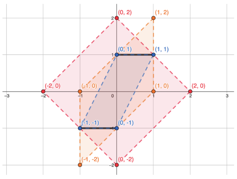
Now, our sensitivity-halving trick from before can be seen as twisting the sensitivity lines along the \(x\)-axis so they end up on top of each other. And this twisting ("linear transformation" if you want to be fancy) allows us to add less noise along this axis. The result is represented in the diagram below. (Note that it also halves the scale of the \(y\)-axis for symmetry, but this has no utility impact.)
The yellow bounding box represents the unit noise. It covers our sensitivity lines, so our algorithm is DP, and it's smaller than the red box from earlier, so the accuracy is better. Can we improve it even more?
Look at the point in the middle of the top line, at (0,0.5). Its sensitivity is 0.5, so some of it is "wasted"! To prevent that, we can rotate our lines by 45°, and stretch them a little, and cover the entire possible area whose \(L_1\) sensitivity is 1. Converting this from the geometric intuition into formulas is left as an exercise for the reader2.
This looks optimal. Is it actually optimal? The authors prove that it is… up to a factor of 2. Clearly they were not happy with this, because the paper keeps going. The sensitivity tweaking is optimal, but it turns out that the noise distribution is not: the authors come up with a better (if somewhat involved) noise distribution, which achieves optimality.
Private Means and the Curious Incident of the Free Lunch
By Jack Fitzsimons, James Honaker, Michael Shoemate, and Vikrant Singhal. Here's a link. Great title, by the way.
This is a different interpretation of the same idea. Say you want to compute the DP mean of a bunch of numbers between 0 and 1, and one of your numbers is 0.1. When computing the sum, hiding this number behind Laplace noise of \(1/\varepsilon\) is, in a way, "wasting" a sensitivity of 0.9. To avoid this waste, you could compute not just the sum of the \(x_i\), but also the sum of \(1-x_i\) as well. A point will contribute \(x_i\) to one sum and \(1-x_i\) to the other, so the total sensitivity of both queries together is still 1! So you can add Laplace noise of scale \(1/\varepsilon\) to both. You get two queries for the price of one.
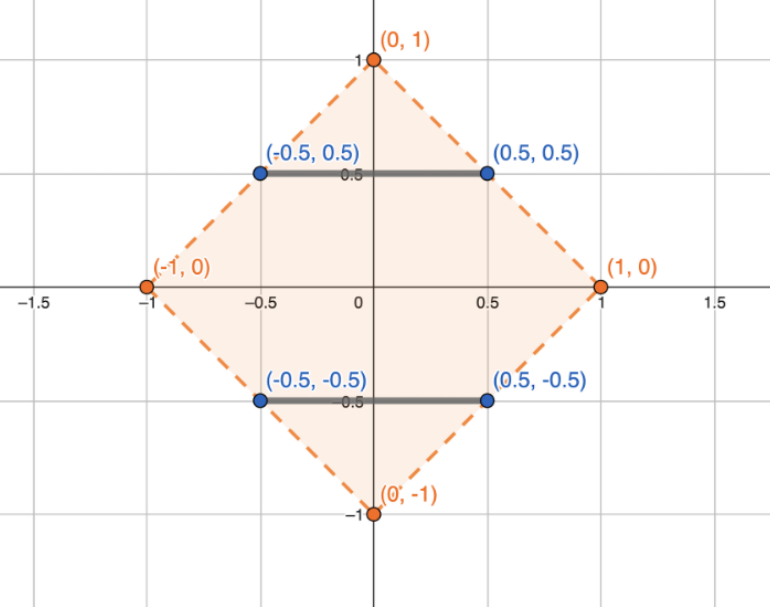
Visually, you're projecting each of your numbers on the line between (0,1) and (1,0). It looks like this (in the figure below, \(R=1\)).
Crucially, if you have a noisy estimate of both the sum of \(x_i\) and the sum of \(1-x_i\), then you can sum both, and get an estimate of the sum of \(1\)… Which is just a noisy count! So to compute your mean, you can use all your budget for the two sums, and get the count for free. Same math than the previous paper, different interpretation ✨
Oh, and you might have noticed that there's also a circle in the figure above. That's because the idea also works with the Gaussian mechanism: the straight line is contained within the unit circle, so the transformation also guarantees that the \(L_2\)-sensitivity is below 1. However, when using Gaussian noise, you often want to use DP variants like like zero-concentrated DP, and add noise to many statistics at once. Can you do better in that case? What a smooth transition to the final paper in this small series.
Better Gaussian Mechanism using Correlated Noise
By Christian Janos Lebeda; here's a link.
Using Gaussian noise is especially useful when a single person can contribute to multiple statistics. So here, we're interested in multiple sum queries, where each person contributes a number between 0 and 1 to each query. And because 2-dimensional math is a lot easier to visualize, we're going to pretend that there are only two queries.
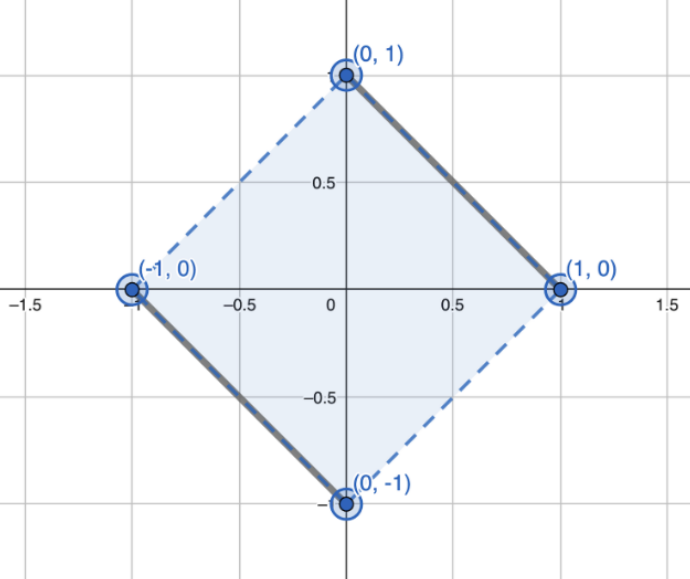
In the add-remove model, what are the possible values of the sensitivity? Either we add an element, in which case both the \(x\)-axis and the \(y\)-axis increase by at most 1. Or we remove one, in which case both axes decrease by at most one. It's impossible for one query to increase and the other to decrease. Just like before, we can represent this on a graph.
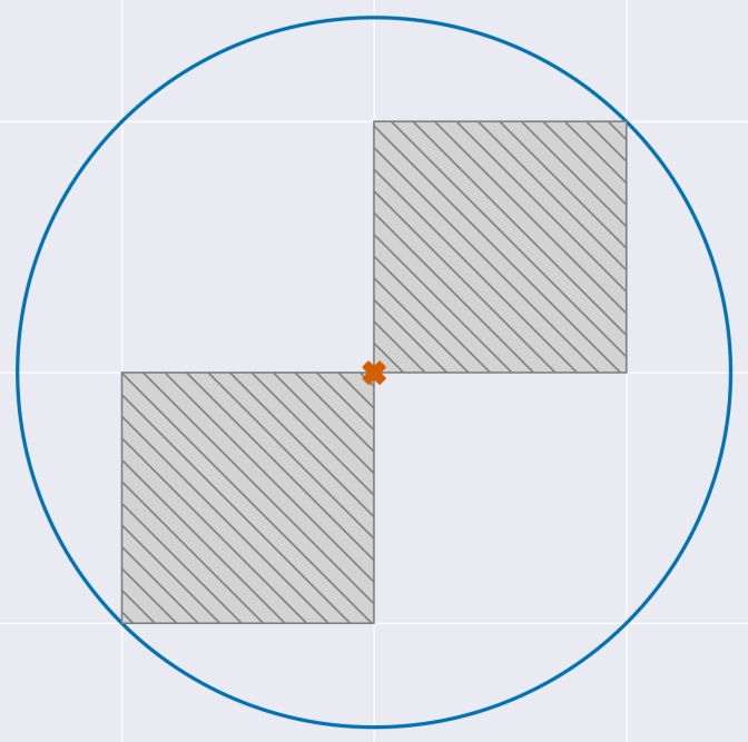
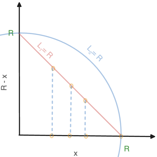
The blue circle represents the Gaussian noise added to the sum. Look at all that wasted space on the top left and bottom right. Very inefficient. What we would really like to do is make the noise fit snuggly with each square, like this.

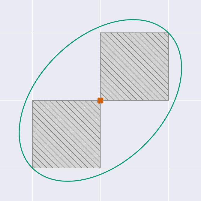
Here, we've added noise centered on (0.5,0.5). This works well to cover one square, but we have to cover both. So the key insight is to also add noise along the \(y=x\) line, in yellow in the diagram above. This second noise component is correlated: we add positive noise to one query if we also add positive noise to the other.
Summing both noise distributions, we end up with a noise shape that looks like this.
And of course, the same idea applies to more than two queries. The more queries you have, the more you benefit from using this technique, which can save you up to a factor of 2 in the noise scale. As a bonus, the author proves that this noise distribution has exactly the same privacy loss as our Gaussian mechanism, which is neat.
A variant on this setting is when you have lots of queries, but each user contributes to a smaller number of queries: for example, if you do a histogram of words used on a search engine, each user will contribute to many words, but much fewer than the total number of words. It turns out that the idea of using elliptic noise, with a component centered on the (1,1,…,1) vector, still works! This is proved in this other paper; the math is more complex and much harder to explain geometrically, but the fundamental insight is the same.
All papers listed in this blog post also have extensions to related problems, and additional results. Go read them if you want to learn more!
Editing note: the first two sections of this blog post were heavily modified after Amit Keinan pointed out a mistake in an earlier version of the Fitzsimmons et al. paper, which I didn't notice and reproduced in this blog post: the technique works for means in the add-remove model, but not in the change-one model. Thanks Amit for letting me know about it!
I'm also grateful to Alex Kulesza and Michael Shoemate for their helpful comments on earlier versions of this post.
-
A bit of a rabbit hole, but if you want to see an example of how easy it can be to get DP wrong even for basic mechanisms, Ctrl+F "Algorithm 2.3" on this page and read until the footnote. ↩
-
Just kidding. You add Laplace noise of scale \(1/\varepsilon\) to the sum of \(x_i\) (call this \(A\)) and the sum of \(1-x_i\) (call this \(B\)), then return \(A/(A+B)\). ↩