Lowering the cost of anonymization

4.2.6 Robustness and testing ✿

Writing bug-free software is notoriously hard. This is particularly problematic when bugs can potentially break the privacy guarantee that a tool is supposed to provide. A well-known example is the attack on the naive implementation of the Laplace mechanism on floating-point numbers [283]: the noisy version of such numbers can leak information on their raw value via their least significant bits. Fixing known vulnerabilities is one thing; but how can we increase our degree of confidence that the software used for important production use-cases correctly enforces its advertised privacy guarantees?

General software development good practices are obviously part of the solution: keeping the design simple and modular is one example, requiring code reviews before any code change is another. In this section, we focus on three types of methods to detect bugs and increase our overall level of confidence in our tooling: manual testing, unit testing, and stochastic testing.

Manual testing

We audited the code manually and found some implementation issues. Some of these issues have previously been explored in the literature, notably regarding the consequences of using a floating-point representation with Laplace noise. Some of them, however, do not appear to have been previously mentioned in the literature, and are good examples of what can go wrong when writing secure anonymization implementations.

One of these comes from another detail of floating-point representation: special NaN (“not a number”) values. These special values represent undefined numbers, like the result of $0 ∕ 0$ . Importantly, arithmetic operations including a NaN are always NaN, and comparisons between any NaN and other numbers are always False. This can be exploited by an attacker, for example using a query like ANON_SUM(IF uid=4217 THEN 0/0 ELSE 0). The NaN value will survive naive contribution bounding (bounds checks like if(value > upper_bound) will return False), and the overall sum will return NaN iff the condition was verified. We suspect that similar issues might arise with the use of special infinity values, although we have not found them in our system (such values are correctly clamped).

Another possible failure mode is overflows and underflows. If sufficiently many large 64-bit integer values are added, the resulting number can be close to the maximum possible 64-bit integer. A single element added can make the result overflow, and the result might be a very small negative integer. If noise addition is implemented in a way that implicitly converts the input into a floating-point number, the resulting distributions of noisy outputs are very distinguishable: one will be almost surely positive, the other negative.

From these two examples, we found that a larger class of issues can appear whenever the user can abuse a branching condition to fail if an arbitrary condition is satisfied (by example, by throwing a runtime error or crashing the engine). Thus, in a completely untrusted environment, the engine should catch all errors and silently ignore them, to avoid leaking information in the same way; and it should be hardened against crashes. We do not think that we can completely mitigate this problem, and silently catching all errors severely impedes usability. Thus, is it a good idea to add additional risk mitigation techniques, like query logging and auditing.

Interestingly, fixing the floating-point issue in [283] can lead to a different issue when using the Laplace mechanism in $τ$ -thresholding. The secure version of Laplace mechanism requires rounding the result to the nearest $r$ , where $r$ is the smallest power of 2 larger than $1 ∕ ε$ . If the $τ$ -thresholding check is implemented as if (noisy_count >= $τ$ ), then a noisy count of e.g. $38.1$ can be rounded up to e.g. $40$ (with $r = 4$ ). If the threshold $τ$ is $39$ , and the $δ$ calculation is based on a theoretical Laplace distribution, then a noisy count of $38.1$ should not pass the threshold, but will: this leads to underestimating the true $δ$ . This can be fixed by using a non-rounded version of the Laplace mechanism for thresholding only; as the numerical output is never displayed to the user, attacks described in [283] do not apply.

Unit testing

A standard practice in software engineering is unit testing: testing a program by verifying that given a certain input, the program outputs the expected answer. Of course, for differential privacy software, the situation is more complicated: since DP requires adding random noise to data, we cannot simply test for output equality. Of course, this does not mean that we should give up on unit testing altogether. Two natural, complementary approaches are possible. We believe that using them both is necessary to write solid, production-ready code.

The first approach is to write traditional unit tests for the parts of the system that do not depend on random noise. For example, the cross-partition contribution bounding presented in Section 4.2.3.0 can relatively easily be put under test: create a fake input dataset and query where each user contributes to many rows, and verify that after the stability-bounding operator with parameter $κ$ , each user contributes at most to $κ$ rows. Similarly, the parts of the system that do more than simply adding noise can be tested by removing the noise entirely; either by mocking the noise generator, or by providing privacy parameters large enough for the noise to be negligible: this is partly how we test operations like ANON_SUM, which clamp their output between specified bounds.

The second approach is to write tests that take the noise into account, by allowing the output to be between certain bounds: for example, we can test that adding noise to $42$ leads to a number between $22$ and $62$ . The tolerance of these tests needs to be carefully calibrated depending on the parameters used in the output, and the desired flakiness of the unit tests: what percentage of false positives (the test fails only even though the code is correct, purely because of improbable noise values) is acceptable. Even with a very low flakiness level (we routinely use values lower than $1 0^{- 20}$ ), such tests can detect common programming mistakes, especially for complex operations. Examples of such tolerance calculations can be found in the documentation of our open-source library [365].

This approach based on tolerance levels is useful, but since we typically want to limit the flakiness probability to very small values, it only provides a partial guarantee that. Furthermore, if these simple approaches can check a number of properties of the software under test, they fail at detecting differential privacy violations, which is the most crucial property that we want to guarantee.

Stochastic testing

While the operations used in the engine are theoretically proven to be differentially private, it is crucial to verify that these operations are implemented correctly. Unit tests can find logical bugs, but it is also important to test the differential property itself. Of course, since the number of possible inputs is unbounded, and differential privacy is a property of probability distributions, it is impossible to exhaustively and perfectly check that the engine provides differential privacy. Thus, we fall back to stochastic testing and try to explore the space of datasets as efficiently as possible. This does not give us a guarantee that an algorithm passing the test is differentially private, but it is a good mechanism to detect violations.

Note that we focus on testing DP primitives (aggregation functions) in isolation, which allows us to restrict the scope of the tests to row-level DP. We then use classical unit testing to independently test contribution bounding. The approach could, in principle, be extended to end-to-end user-level DP testing, although we expect that doing so naively would be difficult for scalability reasons. We leave this extension as future work.

Our testing system contains four components: dataset generation, search procedure to find dataset pairs, output generation, and predicate verification.

Input generation

First, what datasets should we be generating? All DP aggregation functions are scale-invariant, so without loss of generality, we can consider only datasets with values in a unit range $[- r, r]$ . Of course, we cannot enumerate all possible datasets ${[- r, r]}^{S}$ , where $S$ is the size of the dataset. Instead, we try to generate a diverse set of datasets. We use the Halton sequence [186] to do so. As an example, Figure 4.14 plots datasets of size 2 generated by a Halton sequence. Unlike uniform random sampling, Halton sequences ensure that datasets are evenly distributed and not clustered together.

−−000−−000....00240024.4.2.4.2 — Figure 4.14: 256 points in ${[- 0.5, 0.5]}^{2}$ generated with Halton sequences of base 2 and 3.

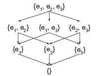
A dataset is a set of records: we consider its power set, and find dataset pairs by recursively removing records. This procedure is shown in Figure 4.15.

pict — Figure 4.15: Dataset search graph for a dataset ${e_{1}, e_{2}, e_{3}}$

DP predicate test

Once we have pairs of adjacent datasets, we describe how we test each pair $(D_{1}, D_{2})$ . The goal is to check that for all possible outputs $S$ of the mechanism $M$ :

P [M (D_{1}) \in S] \leq e^{ε} P [M (D_{2}) \in S] + δ

By repeatedly evaluating $M$ on each dataset, we estimate the density of these probability distributions. We then use a simple method to compare these distributions: histograms.

We illustrate this procedure in Figure 4.15a and Figure 4.15b. The upper curves (in orange) are the upper DP bound, created by multiplying the probability estimate of each bin for dataset $D_{1}$ by $e^{ε}$ and adding $δ$ . The lower curve (in blue) is the unmodified probability estimate of $D_{2}$ . In Figure 4.15a, all blue buckets are less than the upper DP bound: that the DP predicate is not violated. In Figure 4.15b, some buckets exceed this upper bound: the DP predicate is been violated. For symmetry, we also repeat this check with $D_{1}$ swapped with $D_{2}$ .

It is sufficient to terminate once we find a single pair of datasets which violate the predicate. However, since the histogram is subject to sampling error, a correctly implemented algorithm can fail this test with non-zero probability. To address this, we relax our test by using confidence intervals as bounds [384]. We can also parameterize the tester with a parameter $α$ that tolerates a percentage of failing buckets per histogram comparison.

Full algorithm

The overall approach is an algorithm that iterates over datasets and performs a DFS on each of the dataset search graphs, where each edge is a DP predicate test. We present it in the algorithm below. For simplicity, we abstract away the generation of datasets by including it as an input parameter here, which can be assumed to be generated by the Halton sequence, as we described previously. We also do not include the confidence intervals or $α$ parameter described earlier for dealing with the approximation errors. It is also possible to adaptively choose a histogram bin width, but we put an input parameter $K$ here. The general idea is a depth-first search procedure that iterates over edges of the dataset search graph.

Inputs: 
  - mechanism  $M$  
  - parameters  $(ε, δ)$  
  - datasets  $D$  
  - number of samples  $N$  
  - number of histogram buckets  $K$  
Output: whether we found a differential privacy violation for  $M$  
 
for each  $D_{r} \in D$ : 
  // Initialize search stack 
   $S \leftarrow {$  root node  $D_{r}}$  
  while  $S \neq \emptyset$ : 
     $A \leftarrow p o p (S)$  
     $S \leftarrow S \cup {s u c c (A)}$  
    for each  $B \in s u c c (A)$ : 
      // Generate samples 
       $X_{A} \leftarrow {x_{A}^{(i)} \sim M (A) ∣ i = 1, \dots, N}$  
       $X_{B} \leftarrow {x_{B}^{(i)} \sim M (B) ∣ i = 1, \dots, N}$  
      // Determine histogram buckets 
       $H_{min}, H_{max} \leftarrow min (X_{A} \cup X_{B}), max (X_{A} \cup X_{B})$  
       $h \leftarrow \frac{H_{max} - H_{min}}{K}$  
       $B \leftarrow {B_{k} = [H_{min} + (k - 1) \cdot h, H_{min} + k \cdot h] | k = 1, \dots, K}$  
      for each  $B_{k} \in B$ : 
        // Check DP condition using approximate densities over  $B_{k}$  
        if  $∣ ∣ {i ∣ ∣ x_{A}^{(i)} \in B_{k}} ∣ ∣ > e^{ε} \cdot ∣ ∣ {i ∣ ∣ x_{B}^{(i)} \in B_{k}} ∣ ∣ + δ$ : 
          return "likely violation has been found" 
return "no likely violation has been found"

Listing 4.10: DP Stochastic Test

Our actual implementation includes all of the above omissions, including an efficient implementation of the search procedure that caches samples of datasets already generated.

With the above procedure, we were able to detect that an algorithm was implemented incorrectly, violating DP. When we first implemented ANON_AVG, we used the Algorithm 2.3 from [252]: we used our ANON_SUM implementation to compute the noisy sum and then divided it by the un-noised count. Our first version of ANON_SUM used a Laplace distribution with scale $\frac{| U - L |}{ε}$ , where $U$ and $L$ are the upper and lower clamping bounds, which is the correct bound when used as a component of ANON_AVG. However, this was not correct for noisy sum in the case when adjacent datasets differ by the presence of a row. We updated the scale to $\frac{max (| U |, | L |)}{ε}$ , as maximum change in this case is the largest magnitude. This change created a regression in DP guarantee for ANON_AVG, which was detected by the stochastic tester.

−−−0000000000000.2.4.6.0.1.1.2.2...642555 — Figure 4.17: Example histogram comparison for Algorithm 2.3 from [252] with incorrect noise.

Figure 4.17 shows a pair of datasets where the stochastic tester detected a violation of the DP predicate. We can clearly see that several buckets violate the predicate. Once the stochastic tester alerted us to the error we quickly modified ANON_AVG to use the correct sensitivity².

This simple approach can be extended in multiple ways. First, rather than only using randomly-generated databases as input to the stochastic tester, we can also add manual test cases, which we expect to be “edge cases”, like with extreme record values or empty databases. Second, the differential privacy test presented above can be improved using the approach presented in [167], which also provides formal bounds on the probability of errors. Third, differential privacy is not the only property that can be experimentally tested in a similar fashion: we can also test that the noise distribution corresponds to the one we expect, by writing a clean-room implementation of each noise distribution, and comparing both via closeness tests [103].

²In a dramatic turn of events, Alex Kulesza later found that Algorithm 2.3 from [252] is not, in fact, differentially private, even with this sensitivity fix. Consider a database $D_{1}$ with a single values $0$ , and $D_{2}$ with two values $0$ and $1$ . Use $[0, 1]$ as a clamping range. On input $D_{1}$ , the density of the output on $x \in (0, 1)$ is $\frac{ε}{2} exp (- x ε)$ ; while on input $D_{2}$ , it is $ε exp (- 2 ∣ ∣ x - \frac{1}{2} ∣ ∣ ε)$ . When $x$ tends to $1$ , the ratio between the two densities tends to $2$ , independently of $ε$ : this is incorrect for values of $ε$ lower than $ln 2$ .

LINKPREV LINKUP LINKNEXT