Lowering the cost of anonymization

4.2.5  Usability ✿

Designing a differentially private query engine for non-expert use requires a number of considerations beside the design and implementation of the system described in the previous section. In this section, we focus on usability: what makes such a system difficult to use by analysts, and how can we mitigate these concerns.

Automatic bounds determination

One major difference between standard SQL queries and queries using our differentially private aggregation operator is the presence of bounds: e.g., when using ANON_SUM, an analyst must specify the lower and upper bound for each sum input. This differs from standard workflows, and more importantly, it requires prior knowledge of the data that an analyst might not have.

To remove this hurdle, we designed an aggregation function which can be sequentially composed with our previously introduced $\epsilon$-DP functions to automatically compute bounds that minimize accuracy loss. Call this function APPROX_BOUNDS(col).

Without contribution bounds, the domain of an $\epsilon$-DP function in our model spans $R$. Finding differentially private extrema over such a range is difficult. Fortunately, we can leverage two observations. First, inputs to this function are represented on a machine using finite precision; typically 64-bit integers or floating point numbers. Second, bounds do not need to be close to the real extrema: clipping a small fraction of data will usually not have a large influence on the aggregated results, and might even have a positive influence by removing outliers.

Consider an ANON_SUM operation operating on 64-bit unsigned integers where bounds are not provided. We divide the privacy budget in two: the first half to be used to infer approximate bounds using APPROX_BOUNDS(col); the second half to be used to calculate the noisy sum as usual. We must spend privacy budget to choose bounds in a data-dependent way.

In the APPROX_BOUNDS(col) function, we instantiate a 64-bin logarithmic histogram of base 2, and, for each input $i$, increment the $\lceil {\text{log}}_{2}i\rceil$th bin. If we have a total budget of $\epsilon$ for this operation, we add Laplace noise of scale $1∕\epsilon$ to the count in each bin, as is standard for differentially private histograms. Then, to find the approximate maximum of the input values, we select the most significant bin whose count exceeds some threshold $K$. This threshold depends on two parameters: the number of histogram bins $B$, and the probability of a false positive $p$ of an empty bin exceeding the threshold.

The probability that a given bin produces a count above $x$ if its true count is zero is $\frac{1}{2}{e}^{-\mathrm{x\epsilon }}$. Suppose we are looking for the most significant bin with a count greater than $K$. In the APPROX_BOUNDS(col) function, we iterate through the histogram bins, from most to least significant, until we find one exceeding $t$. In the worst case, the desired bin is the least significant bin. This means $B-1$ bins with exact counts of $0$ must not have noisy counts exceeding $K$. Thus, the probability that there was not a false positive in this worst case is:

$$p={(1-\frac{e^{-\mathrm{K\epsilon }}}{2})}^{B-1}.$$

Solving for $K$, we obtain:

$$K=-\frac{1}{\epsilon }\text{ln}\left(2-2p^{\frac{1}{B-1}}\right).$$

For example, $B=64$ for unsigned integers. When setting $p$, the trade-offs of clipping distribution tails, false positive risk, and algorithm failure due to no bin count exceeding $K$ must all be considered. Values on the order of $(1-10^{-9})$ for $p$ can be suitable, depending on $\epsilon$ and the size of the input dataset.

The approximate minimum bound can similarly be found by searching for the least significant bin with count exceeding $t$. We generalize this for signed numbers by adding additional negative-signed bins, and for floating point numbers by adding bins for negative powers of $2$.

Note that there are two possible ways to use this algorithm to automatically generate reasonable bounds: we can either use once over the entire dataset, and use the same bounds in every partition, or use it in each partition separately. There are pros and cons to both approaches. Using it over the entire dataset means that more data is being used, so a smaller fraction of the $\epsilon$ can be used for this operation. Further, for aggregations like sums and counts, it means that the noise magnitude used in each partition will be the same, which makes the output data easier to reason about. On the other hand, using it over each partition separately is better suited for use cases where the magnitude of values varies significantly between partitions.

Providing a measure of accuracy

A ubiquitous challenge for a DP interface is the fact that acceptable accuracy loss depends on the data characteristics, as well as on the problem at hand. We address this by giving analysts a variety of utility loss measures. These utility loss measures can be used in two ways, depending on the scenario in which the differentially private query engine is used.

• If the engine is used to generate differentially private data according to a given strategy, by someone who has access to the raw data, the analyst can try various values of parameters to determine which give the best utility for their use case.
• If the engine is used to allow an untrusted analyst to send queries to a dataset to which they have no access, we can still return a subset of utility metrics without breaking differential privacy guarantees.

There is a profound difference between these two scenarios. Some measures of data loss are useful in both. Since all parameters ($\epsilon$, $\delta$, $\kappa$, etc.) are public, the method and noise parameters used in the anonymization process are not sensitive, and can be returned to the engine client. We could give as much detail as we could; however, in practice, we have found that confidence intervals (CI) are the best way to communicate uncertainty about the results. The CI can be calculated from each function’s contribution bounds and share of $\epsilon$. Importantly, it does not account for the effect of clamping or thresholding. Note that for some aggregations, it might be difficult to compute a CI. For example, averages need to combine the confidence intervals from two sources of noise (the sum and the count), and we do not support CI for quantiles.

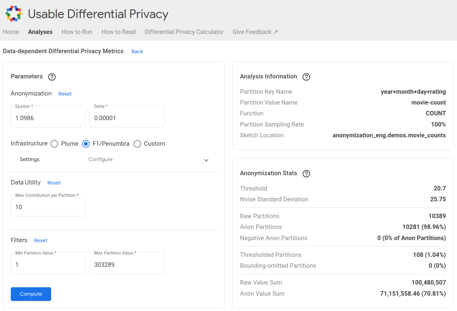
Some measures are more useful in the former scenario, if the analyst has access to the raw data. A particularly useful metric is partition loss: how many partitions with low user counts are removed by $\tau$-thresholding. We can simply return the percentage of lost partitions due to $\tau$-thresholding, possibly as a percentage of all partitions. It would be useful to return this metric in the untrusted use case, but making it differentially private is not straightforward: a single user could add an unbounded amount of partitions, so the sensitivity of this metric is unbounded; and clamping it would defeat the point. This metric is important because it is typically actionable: coarsening the partitions (e.g. aggregating the data daily instead of hourly) can drastically limit partition loss.

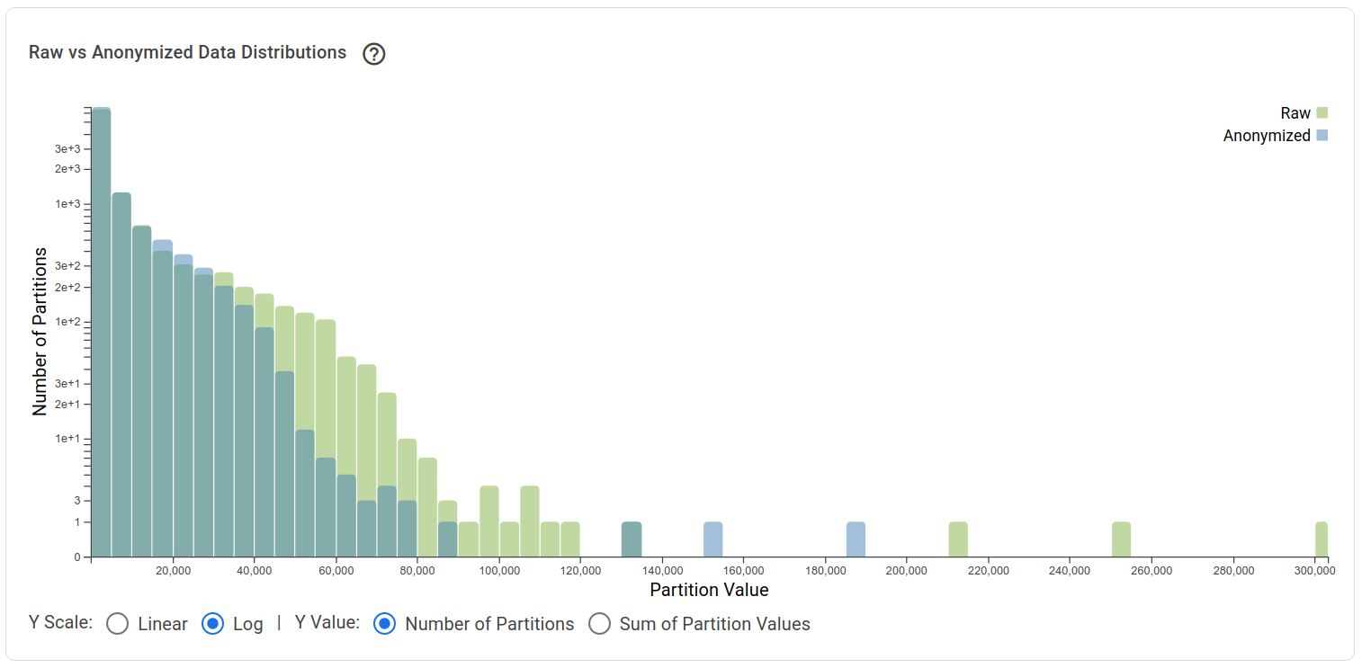
Finally, it is also useful to surface the data loss due to clamping: how many values are clamped, and what is their magnitude. In the “trusted analyst” use case, we can visualize both by simply comparing the private histogram with the non-private histogram, an example is given in Figure 4.13. In the untrusted use case, if we use automatic bounds determination (Section 4.2.5.0), the log-scale histogram gives an approximate fraction of inputs exceeding the chosen bounds; since this is private, it could also be returned to the analyst.

To represent privacy, a techniques and perspectives have been proposed in the literature [200, 234, 243, 290, 304]. In practice, we rely on the prior-posterior explanations and visualizations like those presented in Section 2.1.6.0 to provide an intuitive idea of the guarantees offered by different privacy parameters. This choice is often deferred to privacy experts, we discuss possible approaches to tackling this challenge in Section 4.3.4.0.